Turing Machines

Gregory M. Kapfhammer

September 22, 2025

Simplest possible computer? How to define? Benefits?

• Define the Turing machine
• Explain how it works
• Explore universal computation
• Connect to Python programming

Wait, why not just use Python?

• Python is great for practical programming
• Running a Python program depends on:
  • Operating system
  • Python interpreter
  • Python libraries
  • Hardware architecture
• Completely rigorous proofs require more guarantees
• The Turing machine provides a simple, idealized model

Meet the Turing machine

• What is a Turing machine?
  • Mathematical model: formal definition of computation
  • Simplest computer: only basic operations needed
  • Universal power: can compute anything computable
  • Historical significance: foundation of computer science

• Why study Turing machines?
  • Understand fundamental limits of computation
  • Bridge abstract theory and concrete programming
  • Prove what problems are solvable or unsolvable
  • Foundation for complexity theory and analysis

Turing machine components

• Physical metaphor of a “tape machine”
  • Infinite tape: divided into cells, each holds one symbol
  • Read/write head: can read, write, and move left/right or stay
  • Control unit: finite state machine controlling behavior
  • State dial: shows current state of the machine
• Operations per step
  • Read the symbol under the head
  • Write a new symbol (or keep the same one)
  • Move head left, right, or stay in place
  • Change to a new state (or stay in same state)

A Turing machine is amazingly simple: just tape, head, and state control. Yet it can compute anything that any computer can! Wow, this is incredible!

• Turing machines are “simpler” than real computers
• Yet, they can compute anything that is computable
• Their simplicity allows for deep theoretical insights
• Now, we can mathematically define a Turing machine
• Get ready, this is going to be both challenging and fun!

Formal Turing machine definition

• Alphabet \(\Sigma\): finite set of symbols always including the blank symbol \(\sqcup\)
• State set \(Q\): finite set including start state \(q_0\) and halting/accept/reject states
• Transition function \(\delta\) defined as \(\delta(q, x) = (q', x', d')\)
  • Input: current state \(q \in Q\) and scanned symbol \(x \in \Sigma\)
  • Output:
    • New state \(q' \in Q\)
    • New symbol \(x' \in \Sigma\)
    • New direction \(d' \in \{L, R, S\}\)
• Halting states
  • \(q_{accept}\): halt and computation accepts the input
  • \(q_{reject}\): halt and computation rejects the input
    
  • \(q_{halt}\): halt without acceptance or rejection of input

Simple example: lastTtoA machine

• Goal: Change the last T in a DNA string to A
• Algorithm outline:
  1. Start in \(q_0\), move right to end of string designated by \(\sqcup\)
  2. Move to \(q_1\), scan left looking for a T, which must be the last one
  3. When T is found, replace it with A and then halt the machine
• Examples:
  • CTCGTA → CTCGAA
  • CGAT → CGAA
  • TTTT → TTTA
  • Wait, what would happen with GGGG? We will explain this soon!

Turing machine computation example

Trace of lastTtoA on input CTCGTA:

Step 1: q₀: [C] T C G T A        (start, head at position 0)
Step 2: q₀: C [T] C G T A        (read C, write C, move right)
Step 3: q₀: C T [C] G T A        (read T, write T, move right)
Step 4: q₀: C T C [G] T A        (read C, write C, move right)
Step 5: q₀: C T C G [T] A        (read G, write G, move right)
Step 6: q₀: C T C G T [A]        (read T, write T, move right)
Step 7: q₀: C T C G T A [⊔]      (read A, write A, move right)
Step 8: q₁: C T C G T [A] ⊔      (read ⊔, write ⊔, move left)
Step 9: q₁: C T C G [T] A ⊔      (read A, write A, move left)
Step 10: qₕₐₗₜ: C T C G [A] A ⊔  (read T, write A, stay, halt)

• This simple Turing machine demonstrates key concepts:
  • Reading and processing input
  • Moving the read/write head
  • Producing output by writing a new symbol
• Result: Input CTCGTA becomes the output CTCGAA!

Simple Turing machine simulator

• Map: (state, symbol) to (new_state, new_symbol, direction)
• Next we must define functions to run the machine for an input
• Create simple simulator that any proofgrammer can extend!

Run the simple simulator

Halting and looping

• The lastTtoA machine halts under these assumptions:
  • Input only contains symbols in {A, C, G, T}
  • Input contains at least one T
• What about the input of “CGGA” or “GGGG”?
  • The machine gets stuck in state \(q_1\)
  • The machine will never reach a halting state
• A Turing machine that runs forever is said to loop
• If a Turing machine is not looping we say it halts
• If it halts, then it may accept or reject, or simply halt

Type of Turing machines

• An acceptor accepts or rejects its input:
  • Always halts in either \(q_{accept}\) or \(q_{reject}\)
• A transducer transforms its input:
  • Always halts in \(q_{halt}\)
  • Output is the tape contents when halted
  • Output does not include the blank symbol \(\sqcup\)
• Turing machines can act as:
  • Acceptor or transducer
  • Both acceptor and transducer

The containsGAGA acceptor machine

• Goal: Accept strings containing “GAGA” substring
• Alphabet: {A, C, G, T, ⊔} (i.e., DNA characters and the special blank symbol)
• Machine type: acceptor, not transducer
  • Outputs accept/reject decision, not a modified string
  • Uses states \(q_{accept}\) and \(q_{reject}\) instead of \(q_{halt}\)
• Strategy: scan string left-to-right, track partial matches
• High-level Examples:
  • GAGA → ACCEPT
  • CGAGAT → ACCEPT
  • GATACA → REJECT
  • GGAGAGA → ACCEPT

Understanding containsGAGA states

State meanings for containsGAGA:

• States: \(q_0, q_1, q_2, q_3, q_{accept}, q_{reject}\)
  • \(q_0\): haven’t seen G, or just saw non-G character
  • \(q_1\): just saw first G (i.e., looking for A)
  • \(q_2\): saw GA (i.e., looking for second G)
    
  • \(q_3\): saw GAG (i.e., looking for final A)
  • \(q_{accept}\): found complete GAGA pattern
  • \(q_{reject}\): reached end without finding GAGA

Pattern matching is fundamental to many computational problems. Critically, Turing machines can solve any pattern recognition task!

containsGAGA diagram

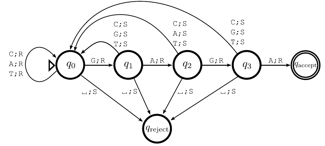
State diagram for the containsGAGA Turing machine.

Acceptor versus transducer machines

• Transducer Turing machines:
  • Transform input string to output string
  • Like functions: input → output
  • Use \(q_{halt}\) state and read final tape contents
  • Example: lastTtoA changes CTCGTA to CTCGAA
  • Like a SISO program that returns an arbitrary string
• Acceptor Turing machines:
  • Make accept/reject decisions about input
  • Like boolean functions: input → true/false
  • Use \(q_{accept}\) and \(q_{reject}\) states
  • Example: containsGAGA accepts/rejects DNA strings
  • Like a SISO program that only returns “yes”/“no”

Simulate containsGAGA in Python

• Simulation of the containsGAGA acceptor Turing machine
• Illustrates pattern matching with state-based memory
• Demonstrates accept/reject computation model for proofgrammers!

The moreCsThanGs acceptor machine

• Problem: Determine if DNA string has more C’s than G’s
• Algorithm strategy: Use cancellation approach
  • Find a G, mark it, look for C to cancel it
  • Find a C, mark it, look for G to cancel it
    
  • If C’s remain after all G’s cancelled → accept
  • Otherwise reject (more G’s or equal counts)
• Examples:
  • CCGG → REJECT (equal counts)
  • CCGGC → ACCEPT (more C’s)
  • CGCGC → ACCEPT (more C’s)
  • GGCCG → REJECT (more G’s)

Simulate moreCsThanGs in Python

Textual representation

q0->q1: x;R
q1->q1: zTA;R
q1->q2: G;z,R
q1->q3: C;z,R
q1->qR: x;S
q2->q2: zTAG;R
q2->q4: C;z,L
q2->qR: x;S
q3->q3: zTAC;R
q3->q4: G;z,L
q3->qA: x;S
q4->q1: x;R
q4->q4: !x;L

• Textbook defines a notation for representing Turing machines
• Save these rules inside of a moreCsThanGs.tm file
• Run in the universal simulator that we later define!

Explain moreCsThanGs.tm

• Compact notation in textbook:
  • Each line represents a transition rule
  • zTA intuitively means “any symbol from {z, T, A}”
  • zTAC intuitively means “any symbol from {z, T, A, C}”
    
  • zTAG intuitively means “any symbol from {z, T, A, G}”
• Why this notation works:
  • z = marker for processed symbols
  • T, A = input symbols to skip over
  • C, G = target symbols for counting/cancelling
  • Encodes the full Turing machine in a text file!

From Turing machines to real computers

• Turing machines are simple but powerful
  • Simulate any computation
  • Extended in various ways
  • Each extension is equivalent in power
  • Python and Turing machines are equivalent!

Chain of simulation approach

• Linux can run any Java virtual machine and
• The Java virtual machine can run any Java program
• Visualization of this chain of simulation:
  • Linux → Java VM → Java program

• Visualization of this chain of simulation for Turing machines:
  • one-tape TM → multi-tape, single-head TM
  • multi-tape, single-head TM → multi-tape, multi-head TM
  • multi-tape, multi-head TM → random-access TM
  • random-access TM → real, modern computer
  • real, modern computer → Python program

Chain of simulation reasoning shows we can simulate a Python program by a Turing machine! Wow!

Multi-tape Turing machines

• Extensions beyond single tape
  • Two-tape machines: separate input and output tapes
  • Multi-tape machines: several tapes for different purposes
  • Two-way infinite tapes: extend infinitely in both directions
  • Multi-head machines: multiple read/write heads per tape
• Why extend the basic model?
  • Makes “programming” more natural and efficient
  • Closer to real computer architectures
  • Separates input, working memory, and output
  • Still equivalent in computational power!

Turing machines to Python programs

• Multi-tape TM → Random-access TM
  • Add random access to any tape position
  • Like having addressable memory locations
• Random-access TM → Real computer
  • Add arithmetic operations and finite memory
  • Modern CPU with RAM and instruction set
• Real computer → Python program
  • High-level programming languages and interpreters
  • The programs we write every day!
• Church-Turing thesis: Every “reasonable” computational model has the same power as Turing machines. Including programs in Python, Java, or C!

Simulating Turing machines

Universal Turing machines

• The ultimate machine
  • Input: description of any Turing machine M and input string I
  • Output: exactly what M would output on input I
  • Universal computation: one machine simulates all others
• How it works
  • Encode machine description as a string
  • Use multiple tapes to simulate M’s computation
  • Step through M’s transitions systematically
  • Universal TM = “interpreter” for Turing machine language

Insight: A single, fixed Turing machine can compute anything that any Turing machine can compute! This is the theoretical foundation of general-purpose computers.

Church-Turing thesis

• The fundamental claim of the thesis:
  • Any function computable by “effective procedure”
  • Can be computed by a Turing machine
  • Informal → formal: bridges intuitive and mathematical computation
• Evidence supporting the thesis:
  • All proposed models equivalent to Turing machines
  • Lambda calculus, recursive functions, cellular automata
  • Modern computers, all existing programming languages
  • No counterexample found in decades of research

For proofgrammers: This means studying Turing machines teaches us about the fundamental limits of all computation, including the Python programs we write!

Python Programs \(=\) Turing Machines

• Every Python program can be simulated by a Turing machine:
  • Apply the chain of simulation approach for:
    • one-tape TM → \(\ldots\) → Python program
  • See textbook for more details about the chain
• Every Turing machine can be simulated by a Python program:
  • Write a Python interpreter for Turing machine descriptions
  • Review the simulator code and check textbook for more details
• Limitations of this approach to equivalence:
  • Turing machines assume an infinite tape
  • Real computers have finite memory

Turing machines for proofgrammers

• Theoretical foundation
  • Formal definition of “computation”
  • Precise statements about solvable/unsolvable problems
  • Mathematical proofs about computational limits
• Practical connections
  • Every Python program corresponds to a Turing machine
  • Algorithm analysis and complexity theory
  • Understanding why some problems have no solutions
• Proofgrammer perspective
  • Bridge between mathematical proofs and executable code
  • Implement theoretical concepts as working programs

Summary: Turing machines as the foundation of computation

• Turing machines are:
  • Simple mathematical models of computation
  • Universal since they can compute anything computable
  • Foundation for understanding computational limits
• Key concepts explored:
  • Formal definition with states, alphabet, transitions
  • Transducers (input→output) versus accepters (accept/reject)
  • Multi-tape extensions and computational equivalence
  • Universal machines and Church-Turing thesis